A multi-class mind tumor grading system primarily based on histopathological photographs utilizing a hybrid YOLO and RESNET networks

Switch studying is extensively utilized in a wide range of contexts. Pre-trained fashions detect easy options like shapes and diagonals within the first layer. Within the subsequent layers, they mix these components to choose up multipart options. Within the remaining layer, the fashions create significant constructs by exploiting options found in earlier phases. We use two well-known fashions to extract options, that are then used to coach the fashions. Determine 2 depicts an summary of the research’s workflow.

With a view to tackle the advanced challenges of mind tumor grading in large-scale histopathological photographs, this work presents a brand new hybrid mannequin that mixes the strengths of three highly effective architectures. By intentionally combining:

• YOLOv5: well-known for its correct and environment friendly object detection capabilities, which permit for the exact localization of tumors inside giant histopathological WSIs.

• ResNet50: a deep CNN with sturdy characteristic extraction capabilities that provides detailed representations of advanced tumor properties required for correct grading.

• XGBoost: an efficient gradient boosting classifier that may additional enhance classification accuracy by capturing advanced non-linear interactions and high-dimensional options inside the extracted options.

This modern mixture presents a number of advantages and constitutes a noteworthy contribution to the sector:

• Enhanced Characteristic Illustration: By combining the strengths of YOLOv5 and ResNet50, a extra complete and insightful characteristic illustration of the tumor is produced, together with contextual and spatial data that’s important for a exact prognosis.

• Improved Grading Accuracy: The thing detection capabilities of YOLOv5 allow correct tumor localization inside the WSI, whereas the deep characteristic extraction of ResNet50 permits the identification of refined tumor traits, leading to improved accuracy for grading activity.

Preprocessing

As a result of complete slide images can’t be dealt with immediately as a result of their huge dimension, some preprocessing processes should be taken. It is usually essential to account for the range in stain colours throughout the dataset whereas ignoring the glass background of the scans. The Open Slide program was used to entry all of the picture slides⁵⁴.

Filtering

WSIs typically have a minimum of a 50% white background, because the white background in WSI evaluation carries no helpful data and might impede classification. Background filtering is a vital preprocessing step. Totally different methods have been tried to do away with the background, resembling coloration thresholding and morphological operations. This mannequin makes use of a simple coloration thresholding approach that examines every pixel’s inexperienced channel values and eliminates any which might be greater than the 200-intensity threshold. When a binary masks is produced, if it covers greater than 90% of the picture, the edge is adjusted till it solely covers lower than 90%. This problem was accomplished utilizing the adaptive non-local means thresholding algorithm⁵⁵. When utilizing H & E-stained histopathological photographs, the place tissue has much less inexperienced content material compared to the white backdrop, this strategy performs properly.

It’s essential to notice that the filtering process may additionally eradicate pixels contained in the tissue space which have a brighter coloration. The median filter, closing filter, and holes filling algorithm had been used to eradicate small holes left by the background filter as a way to clear up this drawback. The filtering process was additionally used on the WSI thumbnails, that are the smallest-resolution representations of the full-sized photographs, to save lots of computing time. The generated binary masks was then upscaled to its full decision. Whereas sustaining the accuracy of the segmentation and classification outcomes, this technique can considerably decrease the computational value of the background filtering process.

Stain normalization

WSIs within the TCGA dataset had been ready at a number of clinics and stained utilizing a wide range of H &E compounds, which may trigger variances in stain colours as a result of environmental components. Stain normalization is thought to be an essential preprocessing step as a result of the variability in stain colours could make it difficult for a neural community to discriminate between GBM and LGG courses⁵⁶. On this research, stain normalization makes use of the Vahadane algorithm⁵⁷, which successfully maintains organic buildings.

In 4 most cancers datasets, Roy et al.⁵⁸ decided that Vahadane’s technique was one of the best coloration normalization approach for histopathology photographs. For normalizing supply photographs with out coloration distortion, the algorithm wants a goal picture. From the unique pictures, stain density maps are generated, capturing the relative concentrations of the 2 stain colours, which offer essential particulars concerning the organic buildings. The goal picture’s stain coloration basis is blended with the density maps to vary solely the colours whereas sustaining the depth of the buildings. The goal picture was chosen relatively arbitrarily to embody a variety of colours from the dataset. Every picture is normalized independently since eradicating the white pixels of the backdrop first is beneficial as a result of they’re merely shaped of the 2 base stain colours.

Patching

One standard technique for getting across the restrictions of making use of neural networks to investigate large photographs is to make use of small patches. Choosing the proper patch dimension is important to steadiness the evaluation’s decision and processing wants. A patch dimension of 1024 x 1024 at 20x magnification is sensible within the context of WSI evaluation for tumor detection because it corresponds to the scale expert pathologists can use to determine tumors. When this dimension is scaled all the way down to the enter dimension anticipated by the vast majority of CNNs skilled on the ImageNet dataset, which is often 224 (occasions) 224 pixels, the world is considerably diminished⁵⁹. Based mostly on these outcomes, the present research tried two patch sizes, small (256 (occasions) 256) and huge (512 (occasions) 512), and efficiently extracted a complete of 225,213 small patches and 40,114 giant patches that didn’t overlap utilizing the tiling approach⁶⁰. To stop analytical redundancy and assure the independence of the patches, it’s essential to make use of non-overlapping patches. We utilized a wide range of augmentation methods to reinforce the range and resilience of the dataset by including to the accessible knowledge samples. A wide range of transformations, resembling rotation, scaling, flipping, translation, and changes to brightness and distinction, had been included in these augmentation methods. Moreover, we used geometric transformations to simulate completely different viewing angles and views, resembling affine transformations.Desk 2 summarizes the variety of extracted patches of varied sizes for every class.

Modeling

This part discusses our Glioma classification algorithms. We apply the two-step approach. The preliminary stage is goal detection utilizing customary approaches, resembling YOLOv5. The picture classifier is used to carry out classifications within the second stage. Much like⁶¹, the choice to make the most of a ResNet50 mannequin was chosen as a result of it has already demonstrated its functionality in medical picture processing. The prediction efficiency of a pre-trained community is in comparison with that of a CNN constructed from scratch on this research.

ResNet50

The residual community is known as ResNet. It types a vital part of the standard laptop imaginative and prescient activity, which is essential for goal classification. ResNet50, ResNet101, and so forth are examples of the traditional ResNet. The problem of the community growing in a deeper route with out gradient explosion is resolved by forming the ResNet community. As is well-known, DCNNs are glorious at extracting low-, medium-, and high-level traits from photographs. We are able to usually enhance accuracy by including further layers. The activation operate of every of the 2 dense layers within the residual module is the ReLU operate. As a result of ResNet-50 presents the advantages of decrease enter complexity, computational effectivity, and pre-trained weight availability, we intentionally selected it over ResNet-152, although the latter could have improved accuracy. By using the optimum depth of ResNet-50 for whole-slide picture evaluation, it was potential to course of a better variety of patches for dependable evaluation and successfully think about particular options of glioma tumors whereas preserving important data. ResNet-50 was chosen as a sensible and efficient possibility for mind tumor grading as a result of it was extremely environment friendly in our coaching course of and gave a powerful basis for characteristic extraction after we used pre-trained ResNet-50 weights.

Deep CNN ResNet-50 has a light-weight design. There are 50 layers that reformulate studying residual features in regards to the layer inputs relatively than studying unreferenced features. The ResNet idea includes a stack of associated or “residual” items. This block represents an array of convolutional layers. An identification mapping path additionally hyperlinks a block’s output to its enter. The channel depth is elevated whereas stride convolution regularly downscales the characteristic mapping to take care of the time complexity per layer.

YOLO

YOLOv5 is a compelling possibility for a reliable and efficient detection mannequin due to its better maturity, ease of use, availability of pre-trained fashions, optimized efficiency for real-time functions, and low useful resource necessities, although there are newer YOLO variations with presumably larger accuracy. As a result of YOLOv5’s structure is much less advanced and requires much less assets than its more moderen variations, it will possibly analyze giant datasets successfully on customary computing {hardware}. That is important for the evaluation of huge quantities of histopathological knowledge with out the necessity for expensive or specialised gear. With a view to analyze giant datasets of histopathological photographs in real-time and enormously improve workflow effectivity, YOLOv5’s pace is essential. Newer variations could also be marginally extra correct, however on this case, their slower inference pace makes them much less helpful. Though there’s a better theoretical accuracy with YOLOv6-v8, YOLOv5 is a extra sensible and superior possibility for mind tumor detection in histopathological photographs as a result of its established presence in medical analysis, pre-trained medical fashions, ease of use, useful resource effectivity, and integration capabilities. With its adaptability to deal with varied tumor varieties with little effort, and its pace and real-time inference capabilities, it is a useful instrument for analyzing giant datasets.

The spine, neck, and head comprise the three important structural elements of the YOLO sequence of fashions. The unique architercture of Yolov5 is proven in Fig. 3. CSPDarknet is utilized by YOLOv5 because the spine to extract options from images composed of cross-stage partial networks. Within the YOLOv5 neck, the options are aggregated utilizing a characteristic pyramid community created by PANet, which is then despatched to the top for prediction. Regarding object detection, the YOLOv5 head has layers that produce predictions from anchor packing containers. As well as, YOLOv5 chooses the next choices for coaching⁶²:

• Leaky ReLU and sigmoid activation are utilized by YOLOv5, whereas SGD and ADAM can be found as optimizer alternate options.

• Binary cross-entropy is used for logit loss because the loss operate

The structure of YOLOv5 mannequin.

YOLOv5 has a wide range of pre-trained fashions. The trade-off between mannequin dimension and inference time is what separates them. Though solely 14MB in dimension, the YOLOv5s light-weight mannequin will not be very lifelike. On the opposite finish of the vary, we have now the 168MB-sized YOLOv5x, which is essentially the most correct member of its household. YOLOv5 options a number of lighting spots over the YOLO sequence, together with:

1. 1.

   Multiscale: To enhance the characteristic extraction community, make use of the FPN relatively than the PAN, leading to a less complicated and faster mannequin.

2. 2.

   Goal overlap: The goal could be mapped to a number of close by central grid factors utilizing the rounding technique.

The elemental function of the mannequin spine is to extract important traits from an enter image. The spine community’s first layer, referred to as the focusing layer, is utilized to hurry up coaching and simplify mannequin calculations. The next targets are achieved by it: The three-channel image is split into 4 slices for every channel utilizing a slicing technique. The output characteristic map was generated utilizing the convolutional layer comprised of 32 convolution kernels. Then, the 4 sections are related in depth utilizing concatenation, with the output characteristic map having a dimension of. After that, the outcomes are output into the following layer utilizing the Hardswish activation features and the batch normalization (BN) layer. The third layer of the spine, the BottleneckCSP module, was created to effectively extract in-depth data from the image. The Layer (Conv2d + BN + ReLu) with a convolution kernel dimension is joined to provide the Bottleneck module, which is the principle part of the BottleneckCSP module illustrated in Fig. 4. The final word output of the bottleneck module is the results of including the output of this portion to the unique enter obtained by the residual construction.

The structure of bottleneck mannequin.

The operation of the CSP community from the primary layer to the final layer is proven by Eqs. 1–3.

the place ([L_0, L_1,ldots ]) means concatenating the layer output, and (W_i) and (L_i) are the weights and output of the i-th dense layer, respectively. Three elements make up the YOLO loss operate: classification error, intersection over union (IOU) error, and coordinate prediction error. The coordinate prediction error reveals the precision of the bounding field’s place, which is outlined by Eq. 4.

the place (lambda _{Cod}) represents the load of the coordinate mistake in Eq. 4. (G^{2}) represents every detection layer’s complete variety of grid cells. N represents the full variety of bounding packing containers in every grid cell. If a goal is current inside the j-th bounding field of the j-th grid cell, (I_{ij}^{T}) will sign this. (bar{a_{i}}, bar{b_{i}}, bar{w_{i}}, and bar{h_{i}}) denote the anticipated field, whereas (a_{i}, b_{i}, and w_{i}, h_{i}) denote the abscissa, ordinate, width, and peak of the middle of the bottom reality, respectively.

The intersection over union (IOU) error reveals how intently the expected field and the bottom reality intersect. Eq. 5 supplies a definition.

The boldness value within the absence of an object is described by the notation “(lambda _{notar})” in Eq. 5. The boldness within the reality and prediction are denoted by (C_i) and (bar{C_i}). In Eq. 6, the time period “classification error” is used to explain the accuracy of categorization.

The found goal’s class is denoted by the letter c in Eq. 6. The real likelihood that the goal is in school c is denoted by the (p_{i}(c)) image. The estimated probability that the goal is a member of sophistication C is denoted by the (bar{p_{i}}(c)) image. So, Eq. 7 represents the definition of the YOLO loss operate.

Improved YOLOv5

The YOLOv5 mannequin’s preliminary implementation doesn’t result in the supposed outcomes. The mannequin ought to precisely determine and classify cancers, even on intricate surfaces. With a view to implement the mannequin in {hardware} gadgets, its dimension should even be as small as possible. We thus modify the mannequin’s skeleton in a number of methods. The YOLOv5 structure’s core community includes 4 BottleneckCSP modules, every having a number of convolutional layers. Despite the fact that the convolution course of could extract image data, the convolution kernel has many parameters, which additionally results in many parameters within the recognition mannequin. The consequence is deleting the convolutional layer on the choice department of the unique CSP module. The enter and output characteristic maps of the BottleneckCSP module are linked immediately by one other department in-depth, considerably reducing the variety of parameters within the module. Determine 5 depicts the structure of the improved BottleneckCSP module. The Optuna library has used to implement hyperparameter tuning for this layer. A abstract of our methodology is offered under:

• Outlined Search House: We created a search house with the next parameters: activation operate (ReLU, Leaky ReLU, Swish), variety of filters (128–192), and kernel dimension (1–3).

• The first goal operate used to evaluate every configuration was validation accuracy.

• Trial Funds: To steadiness exploration and exploitation inside the Optuna framework, we set a trial finances of fifty coaching runs.

The next are the outcomes of the hyperparameter tuning: The very best-performing configuration was decided by Optuna to incorporate 154 filters, a kernel dimension of three, and Leaky ReLU activation.

The entire construction of the mannequin

The RESNET-50 AND YOLOV5 fusion approach makes use of the results of one in every of ResNet-50’s layers as an enter to the YOLO neck whereas combining it with the results of enhanced bottleneckCSP. This ResNet-50 community layer is designated as a characteristic extraction layer in YOLO. On this research, the characteristic extraction layer was primarily based on the ReLU (activation 49 ReLU) layer. The remaining layers of ResNet-50, which embrace the typical pooling, totally related, softmax, and classification layers, are shortened and mixed with the YOLO layer to create a brand new fused community structure for the detection and classification of mind tumors, as introduced in Fig. 1. We processed the supply images earlier than feeding them into YOLOv5 and ResNet50. YOLOv5’s spine was enhanced by the mixing of ResNet50 as a complementary characteristic extractor to realize one of the best characteristic extraction for the classification inside the structure. We acknowledged that the ResNet50 mannequin may seize high-level visible representations, so we initially skilled it with weights pretrained on ImageNet by using switch studying ideas. We tuned the previous couple of layers of the ResNet50 mannequin particularly to satisfy the necessities of our detection activity within the YOLOv5 framework. With a view to fine-tune the community, most of its layers had been frozen, and the weights of the totally related and remaining convolutional layers had been modified. Our aim in fine-tuning these chosen layers was to change ResNet50’s characteristic extraction capabilities in order that they extra intently matched the traits and intricacies current in our object detection dataset. This fine-tuning strategy not solely enhanced the mannequin’s capability to extract advanced visible options pertinent to our activity, however it additionally expedited convergence when the YOLOv5 detector was subsequently skilled. By concatenating the outputs from the YOLOv5 spine with the activations from the ultimate two layers of ResNet50, we carried out a focused characteristic fusion to maximise the strengths of each fashions. With a give attention to semantic richness, the deeper layers of ResNet50 extracted detailed characteristic maps that had been strategically fused into the spatial hierarchy captured by YOLOv5. After this mix, we took a fine-tuning technique, specializing in the joined layers to allow a well-balanced mixture of characteristic representations from each networks. We particularly began selectively fine-tuning the concatenated layers in order that the unique YOLOv5 structure wouldn’t be disturbed, and we may step by step adapt to the specifics of the detection activity. To facilitate a extra custom-made extraction of discriminative options related to the intricacies of our dataset, this fine-tuning primarily concerned modifying the weights and biases of the mixed layers.By way of the method of characteristic concatenation and fine-tuning, we had been in a position to mix the strengths of each ResNet50 and YOLOv5 as a way to maximize their complementary skills. This technique not solely accelerated the mannequin’s capability to seize context and fine-grained visible particulars, however it additionally made improved the classification efficiency potential. XGBoost categorizes the enter knowledge and creates predictions when options from a hybrid mannequin have been extracted. Since XGBoost is best at dealing with high-dimensional options, capturing non-linear relationships, and adapting to completely different tumor displays, we selected them over classical machine studying fashions. This mixture of parameters contributes to the success of bettering algorithms in medical picture evaluation and ensures efficient evaluation and prognosis in medical settings by enabling strong and correct classification of mind tumors in histopathological photographs. By making use of XGBoost as a classifier, we could profit from its capability to handle large datasets and complex characteristic areas, making it a wonderful possibility for this type of activity. Total, the predictions produced by combining XGBoost with ResNet50 and YOLOv5 are extra exact and efficient. Algorithm 1 lists the glioma tumor classification approach primarily based on mind histopathological RGB photographs.

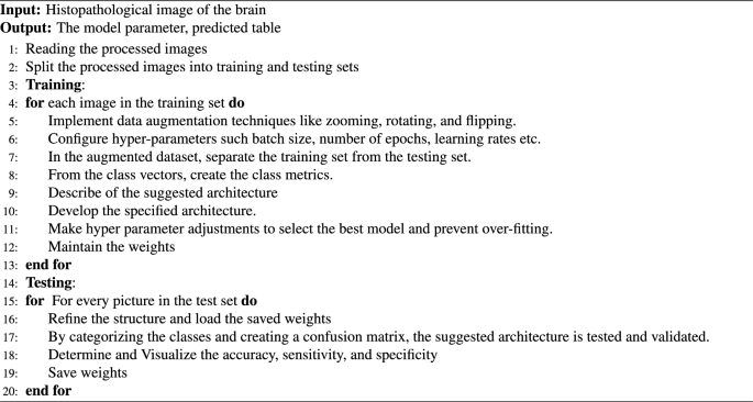
The glioma tumor classification